Changes in Snow Depth, Snow Cover Duration, and Potential Snowmaking Conditions in Austria, 1961–2020—A Model Based Approach


1
Climate Research Department, ZAMG—Zentralanstalt für Meteorologie und Geodynamik, Hohe Warte 38, 1190 Vienna, Austria
2
Department of Geography and Regional Science, University of Graz, 8010 Graz, Austria
3
Department of Geography, University of Innsbruck, 6020 Innsbruck, Austria
*
Author to whom correspondence should be addressed.
Atmosphere 2020, 11(12), 1330; https://doi.org/10.3390/atmos11121330
Submission received: 2 October 2020
/
Revised: 1 December 2020
/
Accepted: 4 December 2020
/
Published: 8 December 2020
(This article belongs to the Special Issue Climatological and Hydrological Processes in Mountain Regions)
Abstract
:We used the spatially distributed and physically based snow cover model SNOWGRID-CL to derive daily grids of natural snow conditions and snowmaking potential at a spatial resolution of 1 × 1 km for Austria for the period 1961–2020 validated against homogenized long-term snow observations. Meteorological driving data consists of recently created gridded observation-based datasets of air temperature, precipitation, and evapotranspiration at the same resolution that takes into account the high variability of these variables in complex terrain. Calculated changes reveal a decrease in the mean seasonal (November–April) snow depth (HS), snow cover duration (SCD), and potential snowmaking hours (SP) of 0.15 m, 42 days, and 85 h (26%), respectively, on average over Austria over the period 1961/62–2019/20. Results indicate a clear altitude dependence of the relative reductions (−75% to −5% (HS) and −55% to 0% (SCD)). Detected changes are induced by major shifts of HS in the 1970s and late 1980s. Due to heterogeneous snowmaking infrastructures, the results are not suitable for direct interpretation towards snow reliability of individual Austrian skiing resorts but highly relevant for all activities strongly dependent on natural snow as well as for projections of future snow conditions and climate impact research.
1. Introduction
The seasonal snow cover (SC) in the European Alps shows strong year-to-year and multi-decadal variations, which are superimposed onto the long-term climate signal, thus partly masking longer-term trends [1]. As a proxy for the energy and mass balance components, both temperature and precipitation changes cause those of the SC, thus resulting in a complex reaction to climate change [2]. Ocean–atmosphere interactions are the main reason for the short-to-medium-term variability of the SC [3]. However, long-term decreasing snow trends in the European Alps, as a response to atmospheric warming, are well constrained by many studies [3,4,5,6,7,8,9,10,11,12,13]. Because of the loss of natural SC and its variability, technical snow production plays a key role today to allow the stable operation of skiing resorts [14]. Currently, about 70% of ski slopes in Austria are equipped with snowmaking [15]. Technical snow is produced by expelling small liquid water droplets from the snow gun through nozzles at high speed. These droplets must then freeze when exposed to the ambient atmosphere. The snow production potential is a function of wet-bulb temperature within the defined limits of −2 °C (upper temperature limit) and −14 °C (maximum water flow in the snow gun) [16]. Due to the temperature dependency of snow production and given natural limits [16,17], the snow reliability of skiing resorts in the future strongly depends upon possible technological improvements and possibilities to increase snowmaking capacities [15,18] but also on a more efficient management of the available snow [19] and water resources [20]. These growing demands are progressively becoming a rising cost factor [21].
In terms of global skier days, Austria is ranked third behind the US and France with a global market share of 15% [22]. The ski tourism sector is estimated to generate EUR 5.9 billion in 2018, representing 1.5% of the Austrian GDP (gross domestic product) [23]. Besides economy, snow has an important role for vegetation (plant species distribution), or water availability (temporal storage), and the climate (feedbacks via short- and longwave radiation balance) [24]. Yet, studies analyzing climate change impacts on the spatiotemporal SC evolution in Austria are sparse [1,25]. Most of these studies are using station recordings of snow depth (HS) and depth of snowfall (HN). There is only one study known to the authors that applies a spatially distributed snow model in Austria to detect area-wide changes [8]. The latter allows us to not only derive highly resolved information in space and time but enables the coupling with climate models to calculate future snow conditions. This is done in the ongoing research project FuSE-AT, this study is part of.
To provide a sophisticated analysis of spatiotemporal changes in past SC conditions in Austria, we use a similar approach as [8] but with a substantially higher number of stations as driving data for the snow simulations, a different SC model, and homogenized validation data. Furthermore, we analyze more target variables of past natural snow changes such as HS, the snow water equivalent (SWE), and the SC duration (SCD) and add the snowmaking potential (SP) as the atmospheric boundary condition for technical snow production. Analyses are performed for seasonal average values of the core winter (December to February—DJF) and the extended season November to April (NDJFMA) based on daily data and include an examination of the elevation dependency of the changes, a regionalization approach, and an investigation of possible forcing mechanisms.
2. Data and Methods
2.1. The SNOWGRID-CL Model
2.1.1. Natural Snow Cover
SNOWGRID [26] is a physically based and spatially distributed snow model, usually applied for operational forecast and driven by gridded meteorological output from the integrated nowcasting model INCA (Haiden et al., 2011). Additional data from remote sensing and in situ stations are used to validate and calibrate the model output. The latter mainly consists of (i) HS and SWE maps in a high spatial resolution of 100 m and a time resolution of 15 min in near real-time and (ii) a 72 h forecast based on the numerical weather prediction (NWP) models ALARO, AROME, and ECMWF used at the Austrian weather service ZAMG (Wang et al., 2006; Seity et al., 2010). SNOWGRID features an energy balance approach with partly newly developed schemes in the INCA system (e.g., for radiation and cloudiness) based on high quality solar and terrestrial radiation data [27], satellite products, and ground measurements. SC physical properties (snow depth, temperature, and density as well as liquid water content for each layer), and SC dynamics are incorporated applying a simple 2-layer scheme. The primary ability of the model is to provide near real time calculations of HS and SWE on spatial high resolution for a wide variety of user needs such as, e.g., avalanche warning [28].
Recently, a climate version of the model, SNOWGRID-CL (SG-CL), has been developed and was applied to historical gridded meteorological data [11]. SG-CL uses an adapted and extended degree-day scheme based on [29] to calculate snow ablation, accounting for air temperature and the shortwave radiation balance. The latter is calculated from clear-sky solar radiation model output [26] and cloudiness derived from daily temperature amplitudes following [29,30] as well as surface albedo (weighted average of snow [31]) and snow-free albedo using CORINE landcover types and albedo values from the literature.
Snow sublimation is calculated from daily potential evapotranspiration fields [32] using precipitation as a dampening factor. It uses a simple 2-layer scheme, considering settling, the heat and liquid water content of the SC, and the energy added by rain and by refreezing of liquid water [26]. For each timestep, SG-CL calculates the following physical SC properties for each of the two snow layers: temperature, density, depth, and liquid water content as well as surface albedo of the upper layer. The daily mass equivalent of HN equals the solid fraction of total daily precipitation sum. The solid fraction of precipitation is calculated using the daily average air temperature in a calibrated hyperbolic tangent function, as there is currently no high resolution observation-based gridded relative humidity information available to derive wet-bulb temperatures, which are the best proxy for the snowline [33]. To convert into HS, fresh snow density is derived from daily air temperature using two different parameterizations, depending on a temperature threshold [34,35]. After daily fresh snow has deposited, the fresh snow added at this time step is considered as a separate layer before it is aggregated to the existing one from former time steps. Next, the SC settles. Settling of the SC is divided into a part that results from destructive metamorphism of the freshly fallen snow crystals (the only settling mechanism for the fresh snow layer) and one that is due to the overburden pressure of the SC. An existing snow layer below the fresh snow layer is applied on both settling mechanisms. The proportion of destructive metamorphism to total settling decreases linearly for snow densities greater than 150 kgm−3. To account for these settling effects, we use the methods described in [36] and used for the SNTHERM89 model; however, we neglect the melting term of the compaction rate.
To correct for precipitation undercatch, an adapted version of the algorithm of [37] is used, with the solid fraction of precipitation and the altitude controlling the magnitude of the correction. Finally, a simple scheme for lateral snow redistribution can be activated in SG-CL based on terrain data and snow density [38]. Thus, the most relevant impacts of wind and humidity processes on the SC energy and mass balance (sublimation and lateral mass transport) are considered by SG-CL. As lateral snow mass transport is one of the main controlling factors for snow distribution in complex terrain, this also addresses the persistence of inter- and intra-annual SC distributions [39,40].
2.1.2. Technical Snowmaking Potential (SP)
SP is defined as the number of hours below a given wet-bulb temperature limit. For the calculation of the spatial distribution of SP by SG-CL on a daily basis, hourly wet-bulb temperatures are estimated from daily temperatures as follows: First, relative humidity are climatologically approximated, then ranked hourly temperatures are estimated from a polynomial curve fit to daily minimum and maximum values using [42] to calculate wet bulb temperatures using the iterative method described in [16]. This also involves a calibration using observed wet-bulb temperatures at representative Austrian sites including the complex terrain. Finally, wet-bulb temperature thresholds varying from −10 to −2 °C (in one-degree intervals) are used to assign hourly SP values (grids) to each calculated hourly wet-bulb temperature. Thereby, the range of SP thresholds is defined by the upper wet-bulb temperature limit according to the actual technology and the temperature of the maximum water flow of the snow guns [16]. In practice, in order to maintain a constant snow quality, the water flow is increased as the wet-bulb temperature of the surrounding air decreases and vice versa. However, different skiing resorts use different thresholds within this range due to different snowmaking technologies, local climate effects, and timing of the winter season (e.g., base-layer vs. reinforcement snowmaking [43]). The produced volume of technical snow could have been calculated as well [16] but is generally a function of the exact technology, manufacturer, and type of snow gun. Thus, on a national scale, SP is used as a much more homogenous measure of spatial and temporal changes in snowmaking conditions.
2.2. Simulation Runs with SG-CL
Recently, high-resolution gridded datasets of daily minimum and maximum 2 m air temperature [44], daily precipitation totals [45], and evapotranspiration [32] have become available for the entire territory of Austria for the period since 1961. Together with the EURO-CORDEX simulations [46], these datasets enabled to generate Austrian climate scenarios (ÖKS15), which include downscaled and bias-corrected [47] grids of daily temperature, precipitation, and global radiation on a 1 × 1 km grid for entire Austria covering the period 1971–2100 [48,49]. The observation-based grids (apart from radiation) are referred to hereafter as SPARTACUS grids and used to drive the SG-CL model for simulating daily SWE, HS, and SP grids at 1 × 1 km horizontal resolution for the winter seasons 1961/62–2019/20. All-sky incoming solar radiation is derived from SPARTACUS air temperature and a solar radiation model (see Section 2.1.1). SCD is derived from daily HS data by counting the number of days with at least 1 cm of snow on the ground in the core winter (DJF) and extended winter season (NDJFMA), respectively. Apart from SP, all calculated variables refer solely to natural snow conditions.
2.3. Trend Analysis and Regionalization
For the detection of trends in the observed and gridded HS, SCD, and SWE time series, we used the nonparametric Mann–Kendall (MK) trend test [50,51]. The latter was applied to seasonal average values of HS and seasonal sums of SCD in the DJF and NDJFMA seasons. The MK trend test is rank based, so that it can also be applied to time series with outliers. Under a given level of significance (e.g., p-value < 0.05), it can be determined from the p-values (two-tailed test) of the MK statistics if, for example, the null hypothesis can be rejected and the alternative hypothesis (meaning there is a trend in the time series) can be accepted. Consequently, the higher the p-values, the higher the probability for no trend in the series. In our study, p-values < 0.05 imply a significant trend in the series, 0.05 ≤ p < 0.1 a tendency and p ≥ 0.1 no significant trend. A trend in a time series strongly depends on the chosen period or the values at the beginning and at the end of the period. In order to account for any possible trend throughout the investigated time period, we use a running trend approach. For this purpose, the window-width for the trend is iteratively increased and moved along the time axis by 1 year. The central value of the time-window is shown on the x-axis and the window-width on the y-axis. Within the resulting triangle, the sign and significance of the trend are shown. The smallest window-width used is 21 years. The strength of the trends is estimated by the Theil–Sen method [52], a robust nonparametric slope estimator for linear regression. For this method, all possible pairs of data (date, measurement) are ordered (from smallest to the largest), connected, and all slopes of lines through pairs of points are computed. The median of all slopes is then the estimate of the strength of the trend (Sen slope).
To validate SG-CL calculated MK trends, we assessed the percentage correct (PC) as a performance measure based on contingency tables of the calculated vs. observed trends at the SNOWPAT sites (major Austrian snow-climate research project, see Section 2.4). PC is defined as the ratio of the sum of correctly calculated significant and not significant trends and the total cases.
In order to investigate possible discontinuities (related to global regime shifts) and trends in the modelled fields, the standard normal homogeneity test (SNHT) [53] and the Mann–Kendall (MK) trend test were applied to the HS, averaged over different elevation sub ranges. Hereby, the elevation range (0–3500 m) is divided into seven sub ranges for 500 m elevation bins. In the SNHT, the time series are tested for a single shift point. The null hypothesis indicates that the series used is homogenous, while the alternative hypothesis indicates that the used series contains a shift point. The sequential MK test [54] is used for determining the approximate starting point of a significant trend. In this test, progressive and retrograde sequential values of the standardized HS (zero mean and unit standard deviation) are computed. Therefore, both series fluctuate around zero. The progressive series is calculated from the first to the last time step (season), whereas the retrograde series is computed backward in time, starting from the end of the series. The intersection of the progressive and retrograde series represents a potential trend starting point within the HS time series. Whenever the progressive or retrograde series exceeds a critical limit, then there is a statistically significant trend, and the intersection point can be considered as the approximate beginning of the trend. In this study, the critical value at the 0.05 significance level is used, which in turn is +1.96 for an upward trend and −1.96 for a downward trend
Finally, we use the moving average over shifting horizon (MASH) analysis [55] to qualitatively detect temporal and seasonal changes in the main meteorological drivers to snow changes, namely air temperature and precipitation taken from the SPARTACUS dataset. The MASH analysis is a filtering method to smooth the high natural variability in the data.
In order to identify regions of different HS variability, agglomerative hierarchical cluster analysis was carried out using the Ward’s minimum variance method [56,57]. In this approach, squared Euclidean distances are used as a measure of similarity. In a first step, the data matrix containing the seasonal (NDJFMA) HS at each grid point is standardized. Next, the standardized data matrix is used to compute a distance correlation matrix, which in turn yields squared Euclidean distances. The Ward’s method starts with n clusters of size 1. Here, n is the number of model grid points. At each step, two clusters are merged that minimizes the increase in the sum of squared distances (variance).
2.4. Validation Data and Methodology
To investigate the robustness of model results with respect to different model approaches, model sensitivity tests were performed, by modifying or switching on/off the following model components: (i) extended vs. simple positive degree-day scheme for snow ablation (with and without consideration of the shortwave radiation balance), (ii) lateral redistribution of snow, and (iii) calibration coefficients of the snow albedo parameterization and the extended degree-day scheme (weighting of air temperature vs. radiation for snow ablation) as well as (iv) the selection methodology of the most representative model grid point. This resulted in 16 different model variants that were compared against observations.
Results of the research project SNOWPAT laid the foundations for the most comprehensive set of homogenized long-term snow observations in Austria with 8 and 40 series beginning in 1901 and 1950, respectively [1]. Follow-up work also demonstrated the relevance of homogenization of snow depth time series for climatological analysis, as the homogenization status influences derived anomalies and climatological trends [58]. The dataset used in our study consists of daily manual snow depth observations, collected by the Hydrographisches Zentral Büro (HZB—national hydrological service) and Zentralanstalt für Meteorologie und Geodynamik (ZAMG—national meteorological service). The dataset of 85 stations until 2019 used for validation in this study is accessible through [59]. Note that the homogenized dataset currently ends in 2011 due to the high workload of the correction process. However, thereafter, a strict quality control was applied.
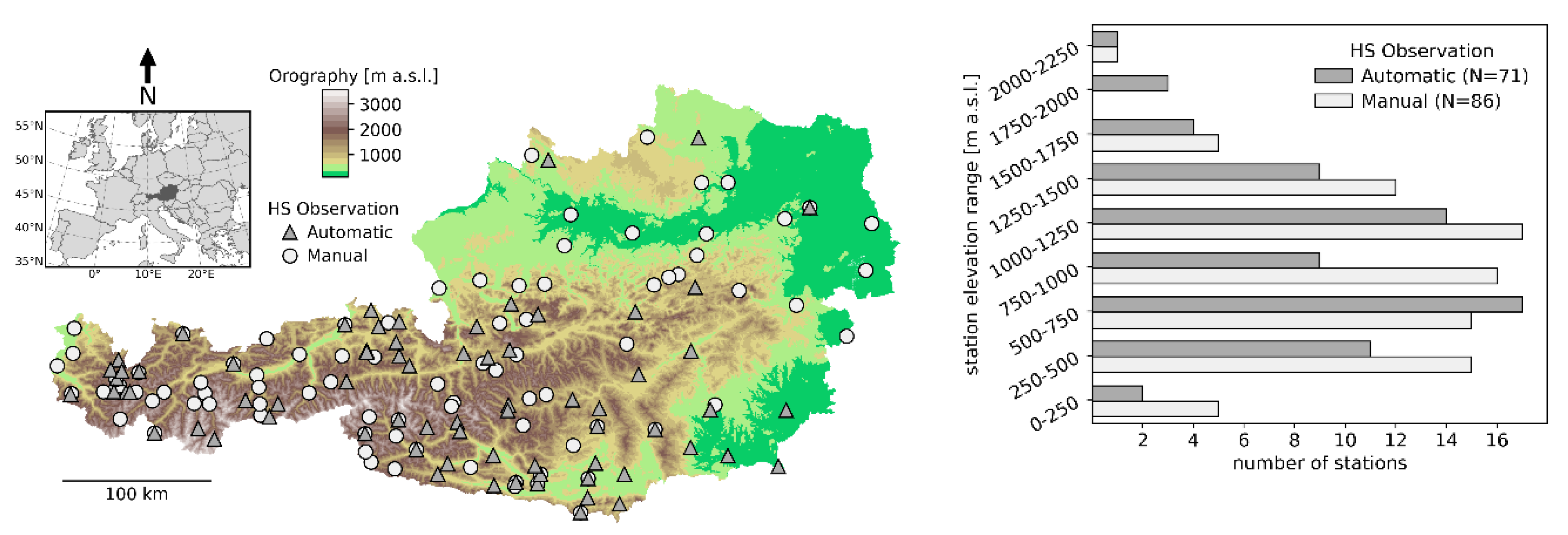
The validation dataset consists of: (a) 85 homogenized long-term manual HS observations, with daily resolution for the period 1961–2019 (SNOWPAT stations in Figure 1), (b) 71 automated laser HS measurements (TAWES stations in Figure 1), 10 min averages aggregated to daily values, for the period 2011–2016. The regional and altitudinal distributions of the stations is shown in Figure 1. Observed SWE data were available for two stations: Maria Alm (1890 m a.s.l., LWD Salzburg) and Kühtai (1970 m a.s.l., TIWAG). Generally, in order to assign SG-CL grid cells to observations, three different approaches were tested: (i) bilinear interpolation, (ii) the vertical nearest grid point of the twelve horizontally closest grid points, and (iii) the average value of the 25th percentile of the twelve closest grid points with a vertical distance of less than 150 m to the observation. The latter approach yielded the best performance measures and was used throughout the validation process.
After calibration of the cloud factor, SG-CL was used to calculate daily global radiation sums, which were compared against measured values at 118 routine measurement sites (TAWES) using a Schenk Star Pyranometer in the independent validation period 2000–2016. Measured snow albedo values using a Kipp&Zonen CNR4 Radiometer at seven stations were compared against calculated values in the period 2014–2017. All measured albedo values have undergone a strict data quality control following the guidelines of the Baseline Surface Radiation Network (BSRN) [60]. Finally, hourly observed vs. calculated wet-bulb temperatures from daily values were evaluated at 44 TAWES stations.
To assess the potential of SG-CL to simulate spatial snow patterns, fractional SC data from MODIS (FSC) provided on a daily basis with a spatial resolution of 250 m by [61] were used for validation over the period 2011–2016. First, days with cloudiness >50% over the model domain were filtered out (leaving a total of 600 days for comparison), and the data were rescaled to the 1 KM resolution of the SG-CL model grid using a nearest neighbor interpolation. In a next step, both SG-CL HS, and the MODIS data were converted into binary SC by applying a threshold of HS = 1 cm and FSC = 15%, allowing the calculation of statistical parameters using contingency tables such as the Kuipers Skill Score (KSS).
3. Results
3.1. Validation Results
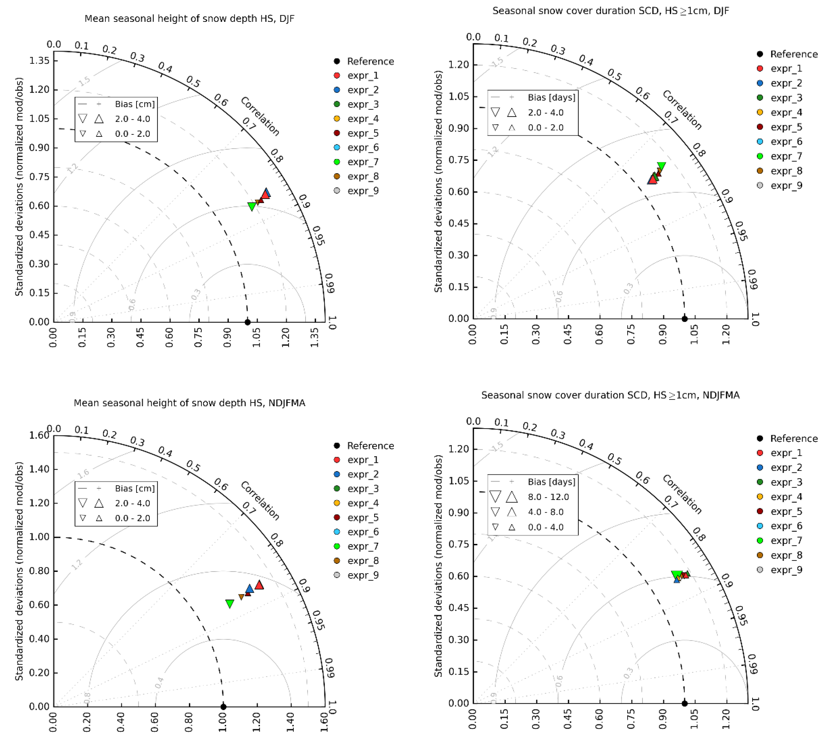
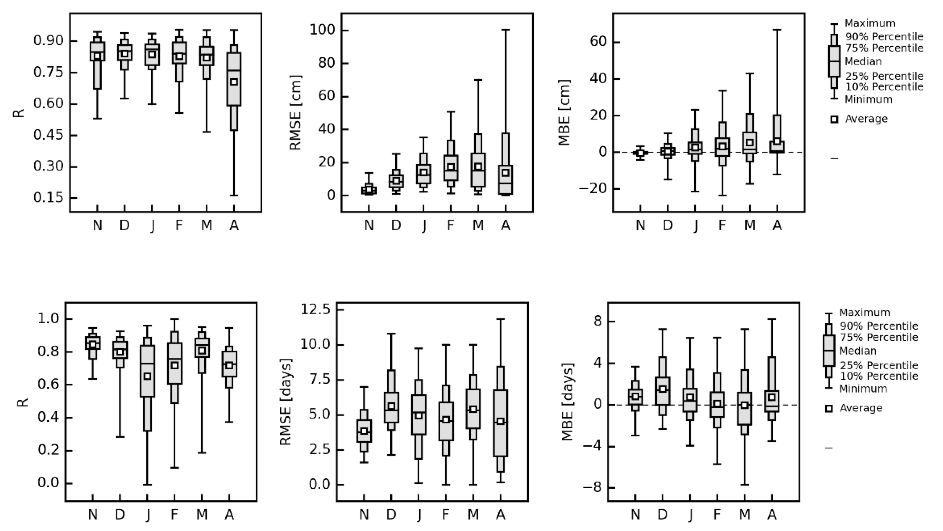
Sixteen different model variants were tested in order to find an optimum SG-CL model setup. The quantitative results of the comparison are shown in Figure 2 for a subset of the variants (model components (iii) in Section 2.4). Using an objective ranking methodology (largest number of rank 1 counts across all performance measures and variables), the best setup was identified (“expr_1” in Figure 2) and used for all further snow simulations. The performance measures of this reference run against the in situ observation subsets are given in Table 1. Compared to the in situ observations dataset, the correlation coefficient (R), the root mean squared error (RMSE), and the bias (BIAS) for seasonal HS (NDJFMA) equal 0.86, 10.23, and 2.86 cm, respectively. In order to limit the average BIAS, the undercatch correction of precipitation was only applied to grid points above 1500 m a.sl. At a monthly time scale (Figure 3), the SG-CL HS simulations show a high correlation of 0.86 to the observations for November to March. In April, the correlation spread increases dramatically and the mean correlation drops to 0.7. Furthermore, the RMSE and BIAS increase from November to April. This is an indication that too high snow depths are simulated during the winter months. In contrast, the monthly performance measures for the snow cover duration show a more variable picture. The mean of the correlation coefficients is in the range of 0.72 to 0.85.
An example time series of SG-CL calculated vs. observed mean seasonal snow depths and SCD is shown for the Station Feuerkogel in Figure 4. Clearly, SG-CL reproduces the observed annual and decadal variability in snow depth and snow cover duration reasonably well.
The multiyear spatial validation against MODIS FSC data result in a probability of detection for snow (POD), false alarm rate for snow (FAR), and Kuipers Skill Score (KSS) of 0.76, 0.41, and 0.69, respectively. Whereas POD and KSS indicate a generally high agreement, the FAR value points to a simulation weakness, when analyzed on a seasonal base, of an erroneously simulated early winter SC that is not observed in reality (the FAR for no snow is <0.1). The reason is that frequent relatively warm ground temperatures in late autumn and early winter are not accounted for in the model (no ground heat flux), and the buildup of a SC is solely controlled by solid fraction of precipitation and its amount (see discussions).
Daily sums of global radiation were calculated with a BIAS of 0.17 kWhm−2 and a RMSE of 0.42 kWhm−2 on average, the latter corresponding to a normalized value of 13%. Observed snow albedo could be reproduced with a squared correlation coefficient of 0.92 and an RMSE of 0.11 (29% normalized). Finally, hourly observed wet-bulb temperatures were approximated with an R2 = 0.9, a BIAS of −0.3 °C, and a RMSE of 1.3 °C.
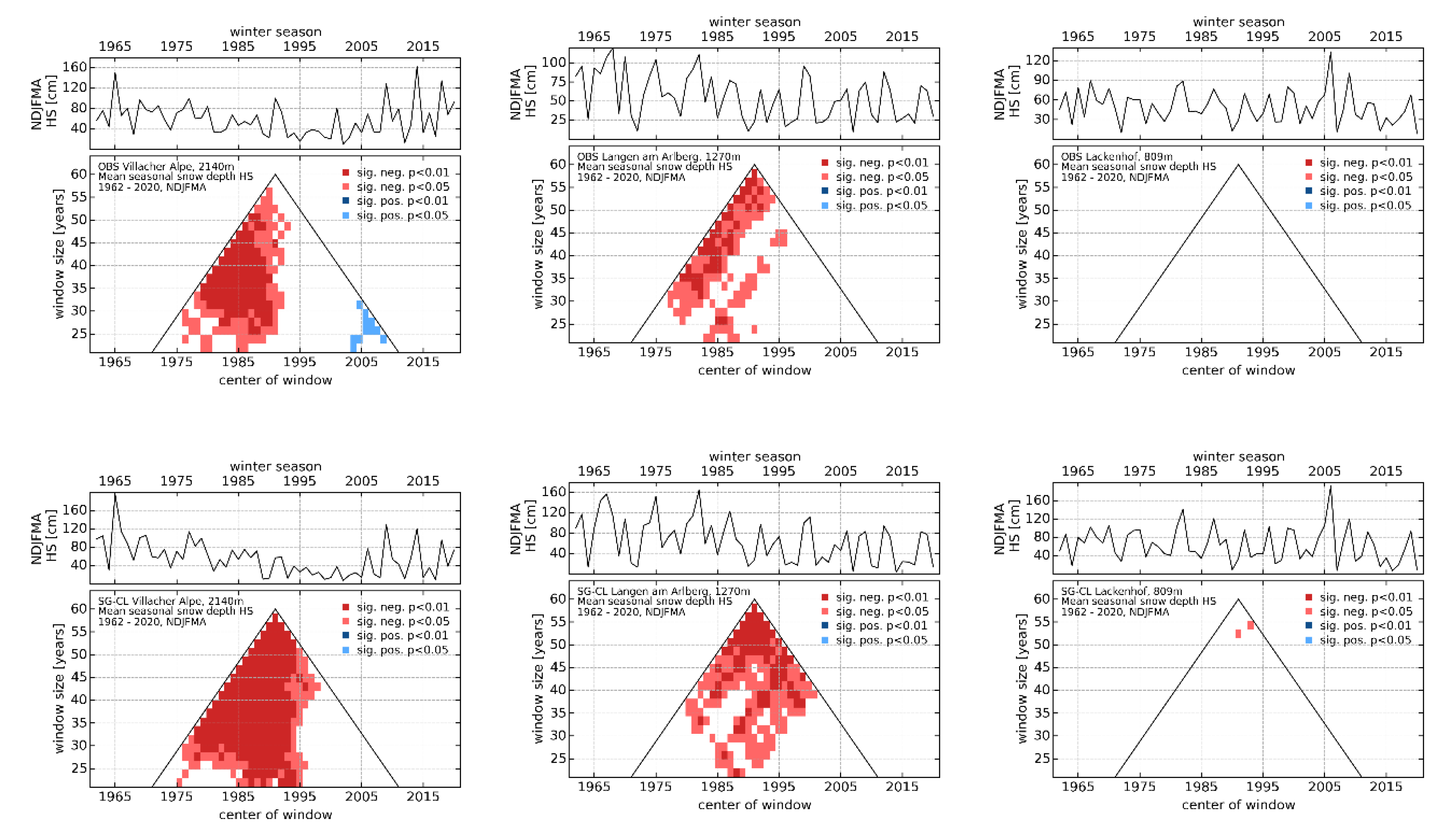
A validation of the running trend analysis finds a PC value of 86% on average over 85 stations in the period 1961/62 to 2019/20 (see Figure 5).
3.2. Past Changes in Natural Snow
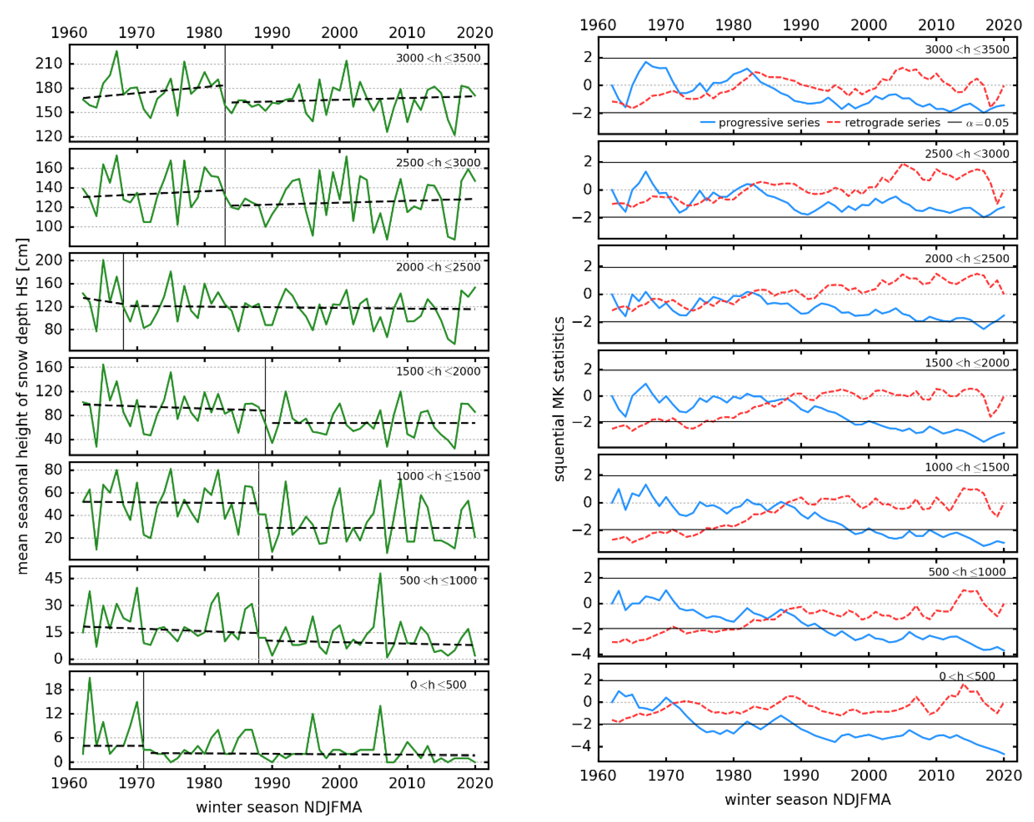
Figure 6 (left) shows SG-CL calculated seasonal HS (NDJFMA) averaged over the seven elevation sub ranges for the seasons of 1961/62 to 2019/20. The visual inspection reveals a high annual and decadal variability. Besides that, a long-term decrease in HS in all elevation subranges can be observed. The statistics of the shift point analyses and the MK trend test are summarized in Table 2. The results of the SNHT suggest that the detected shift points in elevations above 2000 m are not significant at a 95% confidence level. In contrast, significant abrupt changes in HS in the elevation range of 500 to 2000 m occurred during the end of the 1980s. In the lowest elevation range, the significant shift season is 1971. In all elevation subranges, the MK-trend statistics of the subseries (before and after the shift point) indicate the absence of significant trends. However, significant downward trends are detected in the elevation ranges below 2000 m for the whole time series. Figure 6 (right) shows the results of the sequential MK test. The progressive and retrograde series in elevation sub ranges above 2000 m show multiple intersection points, which is an indication for the absence of a significant trend (high temporal variability and mostly cold enough for snowfall). This is true for the long-term time series. The last intersection point in the highest three subranges is 1983. Starting from this point, the progressive and retrograde series are diverging more or less, and the declining progressive series exceeds the critical value (−1.96) only once in 2017. Thus, 1983 can be considered as the significant trend turning point within the time series from 1961/62 to 2016/17, but the trend is nonsignificant for the time series of HS from 1961/62 to 2019/20. Especially, the winter seasons of 2015/16 and 2016/17 were characterized by exceptional low snow depths. It should be noted that the global average surface temperature was the warmest in 2016 since the late 1800s. Furthermore, the sequential MK test for the elevation sub ranges between 500 and 2000 m clearly identifies the season 1988 as the beginning of the significant negative trend in the HS time series. In the lowest elevation sub range, it is 1972. As a matter of fact, the results indicate major shifts of HS around the 1970s and in the late 1980s, which are predominantly responsible for detected negative trends. These shifts are most likely related to the observed global regime shifts in the 1970s and 1980s [9,62].
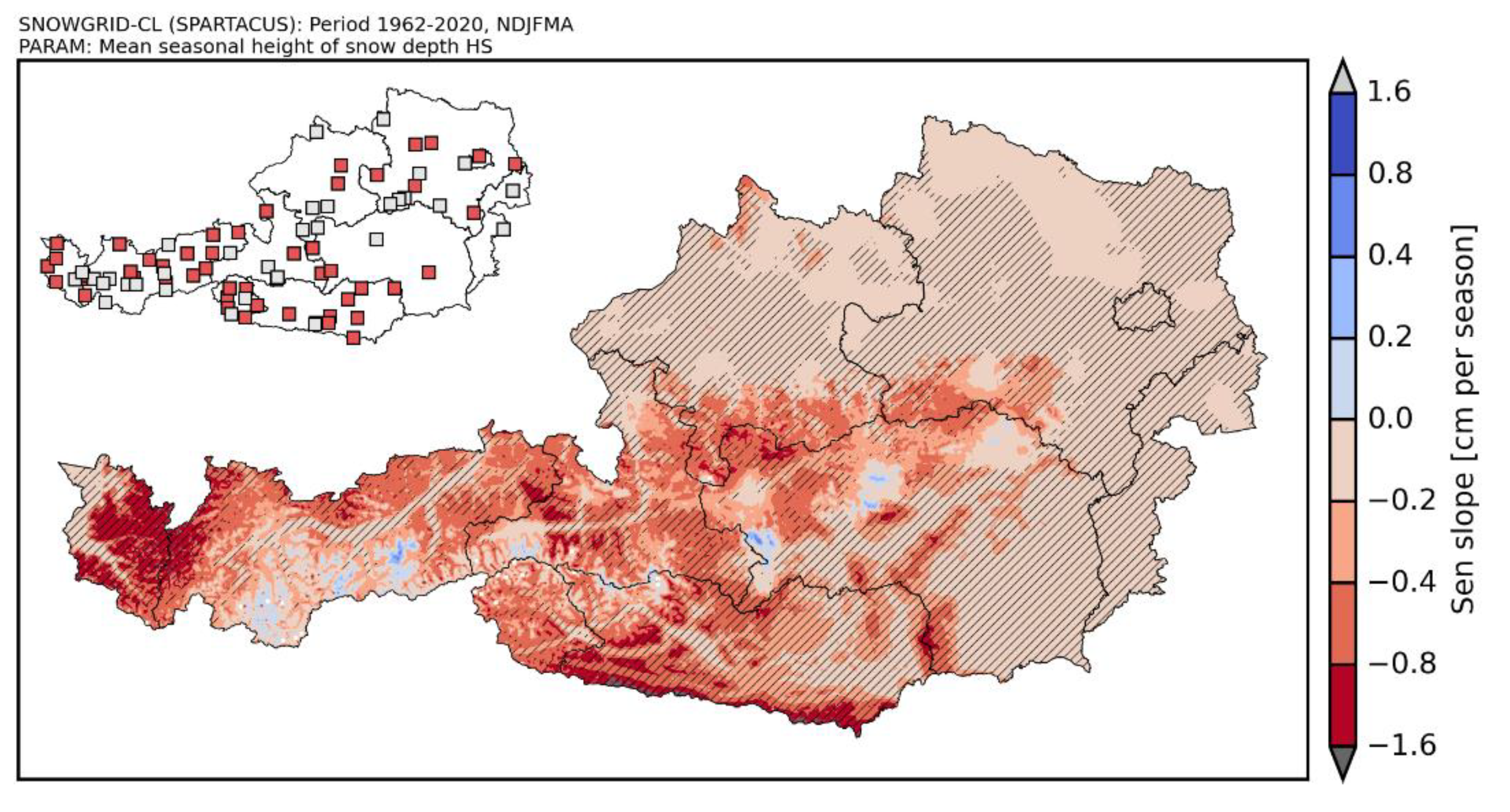
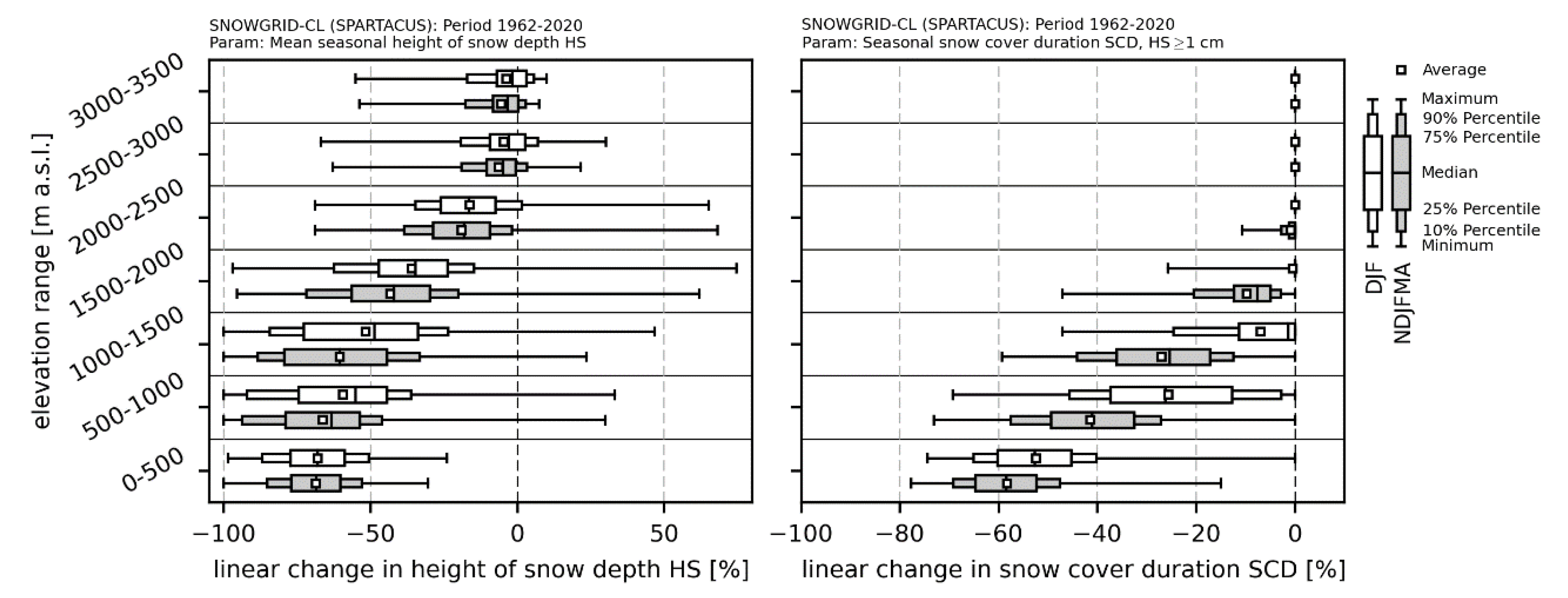
The spatial MK trend analysis for the period 1961/62–2019/20 indicates significant long-term decreases in seasonal average HS and SCD in the extended winter season (NDJFMA) especially in southern and western Austria as well as partly in central Austria (see Figure 7). This general pattern is in good agreement with the results of [1] based on observations, an updated dataset of which is shown as inlet in Figure 7 (top left corner). In absolute numbers, the seasonal average SD and SCD decreased significantly by around 15 cm and 42 days in the period 1961/62 to 2019/20 on average over Austria, respectively. For seasonal maximum HS, the trend patterns and magnitudes are very similar. Decreases in HS in Austria are visible at all altitudes up to 3500 m a.s.l. on both the core and the extended winter season as shown in Figure 8 (left). Absolute HS reductions are largest in mid elevations of about 1800 m a.s.l. and decrease below and above (not shown). Relative HS shrinkage decreases with increasing altitude (−75% to −5% and less than 50% decrease above 1000 m a.s.l.). For absolute and relative SCD trends (Figure 8, right), there is a strong linear altitude dependence with strongest reductions of −55% in the lowest elevations to −10% in 1500 m a.s.l. and no change above 2000 m a.s.l. Some positive outliers in the altitude ranges above 500 m a.s.l. result from the positive tendencies indicated by the bluish areas in Figure 7. Decreases larger than 80% in the total period are only observed in southern Austria. Besides long-term warming, this is also due to a decreasing frequency of southwesterly weather patterns and thus precipitation from the end of the 1980s until around 2003 [1]. The shortening of SCD is due to an earlier melt out of the SC in spring more than a later onset in autumn. The altitudinal profile and seasonal shortening pattern of simulated SCD changes is also in very good agreement with observations [6,25]. Seasonal cumulative fresh snow sums also show a general significant decreasing long-term term trend in most regions apart from northern Austria. Seasonal maximum 72 h fresh snow amounts that are relevant for avalanche formation show a similar long-term decreasing pattern with some regions around the eastern Alpine main ridge (e.g., Dachstein and Hochschwab) that indicate positive tendencies.
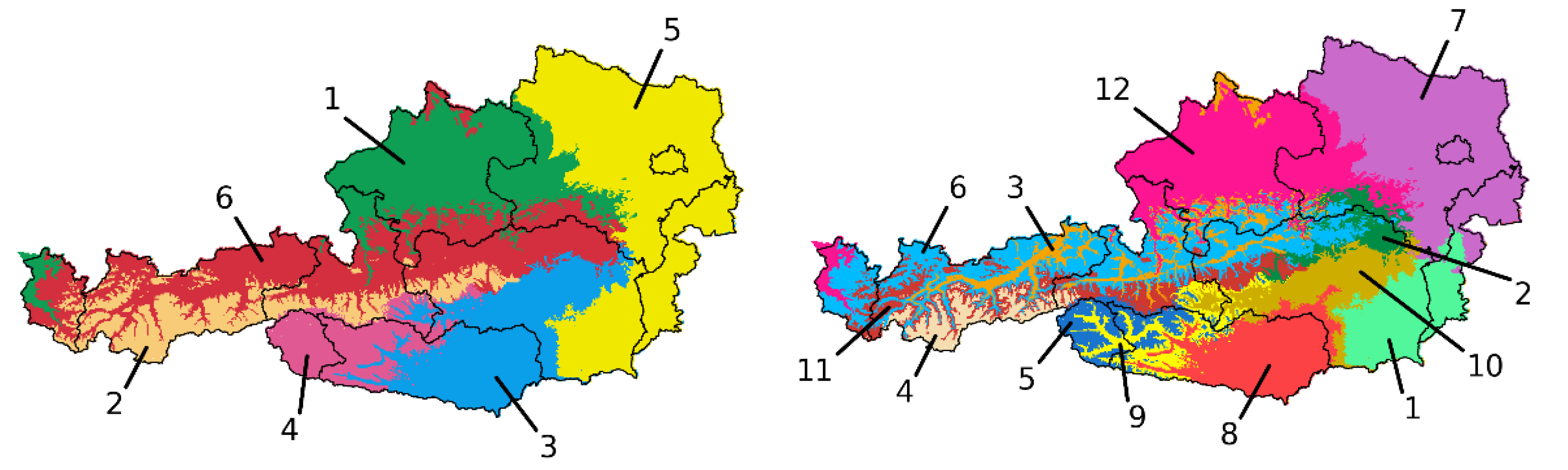
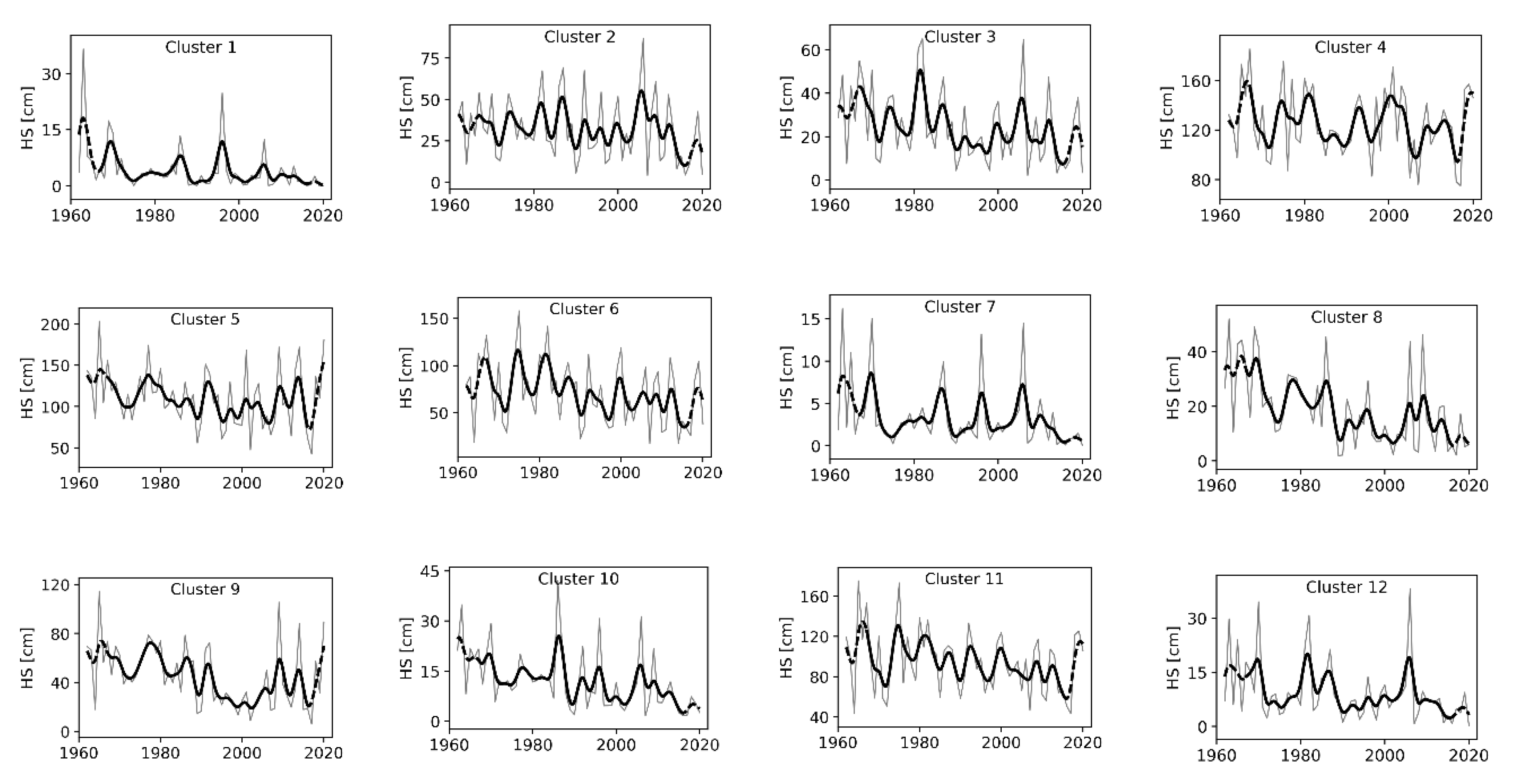
The results of the agglomerative hierarchical clustering analysis using Ward’s minimum variance method are shown in Figure 9. The investigation of the minimum distances between the combined clusters suggests 6 homogenous groups in terms of similarity (elbow diagram, not shown). However, the selection of the optimal number of clusters is heuristic. An accepted objective criterion for the selection of clusters does not exist. In Figure 9, the clustering based on 12 clusters is shown as well. The identified regions are empirically plausible. The use of more clusters minimizes the generalization of information and leaves more room for interpretation. In addition, it gives a detailed picture of the regional variability of HS (see Figure 10). Table 3 and Table 4 summarize the characteristics of the cluster decision with six and 12 groups. The averaged time series of the highest located regions associated with cluster 4, 5, and 11 of the 12-group cluster decision show no significant trends, compared to the lower regions. In all remaining regions, a significant downward trend is detected. Furthermore, all regions are characterized by distinct annual and decadal variability (see Figure 10). A pronounced shift towards lower snow depths is visible in the cluster regions 3, 8, 9, 10, and 12 at the end of the 1980s (mean elevation range of 522 to 1474 m). Besides that, a step change is also visible in 1, 7, 8, 10, and 12 during the 1970s (mean elevation range of 355 to 970 m). In contrast to those findings, cluster 2 shows a quite different variability. The visual inspection reveals an upward tendency until 2010. The historical variability of observed snow depths at climate stations (SNOWPAT stations) located within the clusters are on average in good agreement with the individual cluster variability (not shown).
3.3. Past Changes in Snowmaking Potential
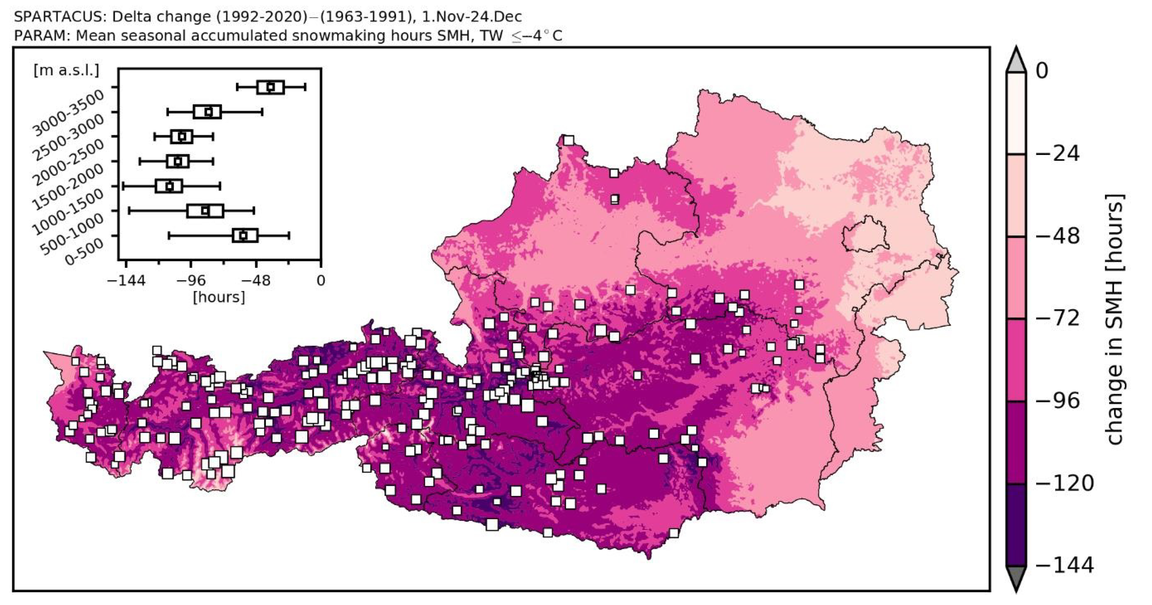
Sustained long-term warming in all seasons and altitudes leads to increased wet-bulb temperatures as well [25] and thus to reduced snowmaking hours and SP. The latter is shown in Figure 11 for one threshold temperature comparing the periods 1991–2020 vs. 1961–1990 during the most important snowmaking time of the year, namely 1 November to 24 December. On average, over Austria SP reduces by 85 h (−26%) between these periods. The changes span a range of −12 to −146 h (−1 to −50%). Strong absolute reductions are found in lowest elevations of some regions such as along the valleys of the Salzach, of eastern Tyrol and parts of upper Carinthia with values between −75 and 100 h. The vertical profile of changes indicates that strongest reductions are found in medium elevations of 1000 to 1500 m a.s.l.
3.4. Meteorological Drivers for Past Snow Changes
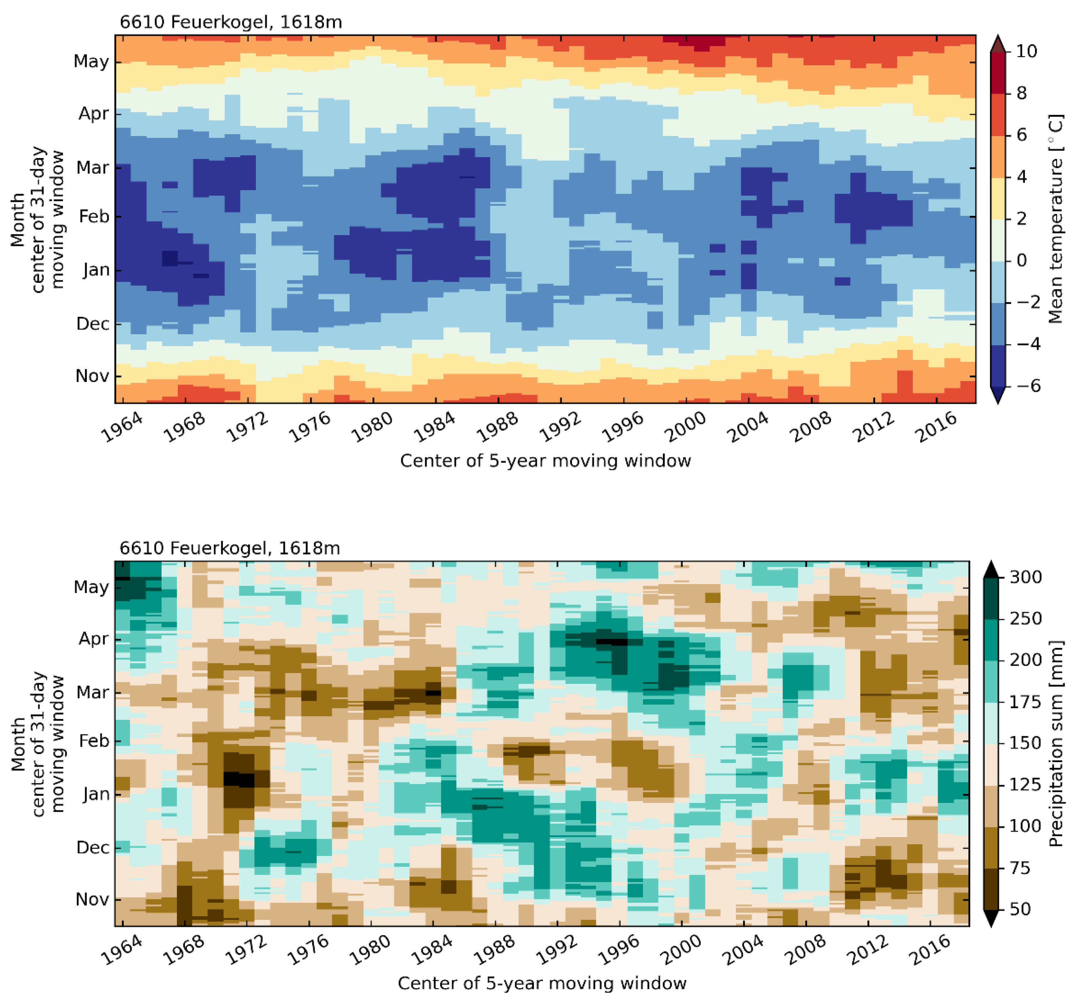
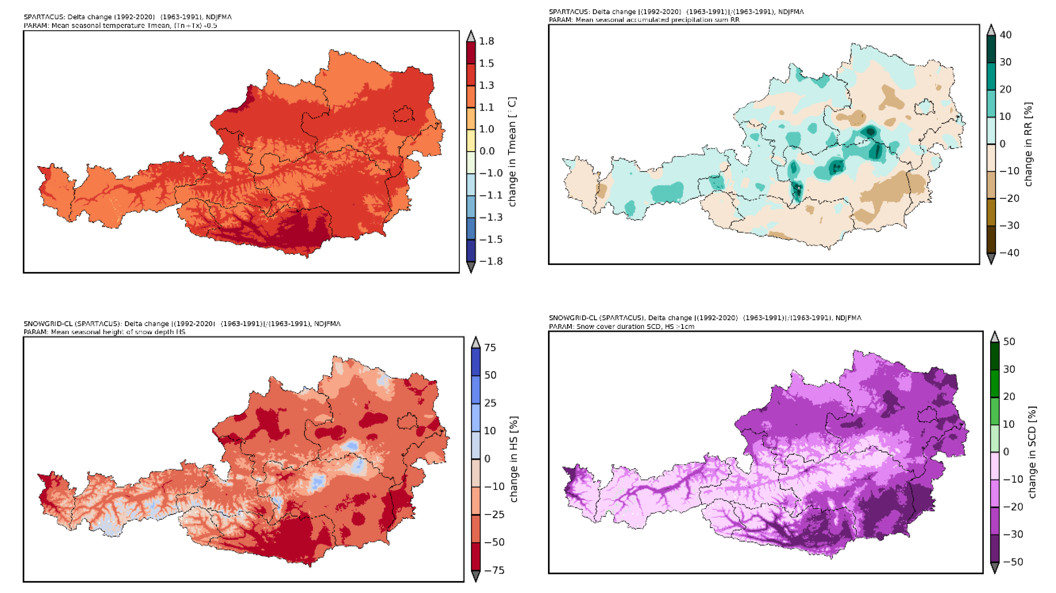
Past observed natural snow changes are mainly driven by changes in air temperature and precipitation. The MASH analysis of temperature and precipitation changes in Figure 12 for a selected point (station Feuerkogel) underlines the strongest temperature increases in spring leading to the observed earlier melt out of the natural SC (see Section 3.2.). The analysis of the precipitation shows no monotonic upward or downward tendencies. Figure 13 allows us to attribute observed snow changes to spatial patterns of air temperature and precipitation changes. Air temperature increased rather homogenously across Austria with maximum increases in low elevations of southern Austria. Precipitation increased significantly from Tyrol (western Austria) eastwards along the Alpine main ridge to the eastern border of the Alps with strongest increases in northern Styria and southern lower Austria (Mostviertel) and decreased in all other regions. The latter leads to weaker snow reductions in parts of these regions. Generally, as cumulative fresh snow sums also decrease (not shown), SC recession is due to the combined temperature effect of increasing liquid fraction of precipitation and stronger melt of snow on the ground. Changing precipitation totals either reinforce or weaken this long-term effect. In higher elevations, temperature sensitivity of snow decreases, and above around 2000 m a.s.l., its most of the time cold enough for snowfall during wintertime, which is corroborated by the shift point and cluster analyses. In this altitude, snow will also depend in future more from precipitation and thus weather patterns [1,64]. Past absolute SP changes are strongest in regions with the coldest temperatures intersecting with the strongest temperature increases.
4. Discussion
Although forced with gridded observational data, SG-CL model errors of SCD and SWE are within a range known from many other more and less complex snow models [65]. Using another SC model and a reduced set of meteorological input data for Austria, the study of [8] found a decrease in SCD in the period 1980–2009 vs. 1950–79 of 11–15 days (8–17%), depending on the regions. We explain the larger decreases found in our study through the more recent periods used with enhanced rates of temperature increase observed and to the more extensive meteorological dataset (150 (70) and 523 (59) temperature and precipitation stations in our study (study of [8]), respectively). The latter also leads to more robust results in complex terrain.
The simulated SCD decrease of 42 days in the period 1961/62 to 2019/20 on average over Austria corresponds to a rate of −7 days per decade, which is 40% above the global average value of −5 days per decade but well within the likely range from 0 to −10 days per decade [66] and very close to the value of −8.9 days per decade found by [6] for eleven stations in Switzerland based on the period 1970–2015. In agreement with our simulation results and observations, the latter is due to an earlier melt out in spring more than to a later snow onset in autumn driven by reinforced warming in the spring season.
Without activation of the lateral snow redistribution scheme in the SG-CL model, snow towers are forming at single, high-elevated grid points due to the piling up of snow over the years as found in other studies [38,67] already. This strongly and unrealistically increases melt rates in these altitudes, as snow is still present during summer months. The location of these gridpoints coincides with accumulation zones of existing glaciers. However, the activation of the lateral snow distribution scheme does not improve the simulation of high-altitude snow masses in wintertime as compared to long-term observed glacier winter mass balance measurements, which are still negatively biased in model simulations. We tentatively attribute this to the simple parameterization scheme (no wind information) and the too coarse horizontal grid resolution of 1 km, which leads to a smoothing of terrain features essential for correct lateral snow transport and deposition. High-resolution model runs with 100 m grid size as used for the operational SNOWGRID version could be constructive in this regard. The second reason for underestimation of high-altitude snow mass are undercatch errors contained in the precipitation grids. The algorithm that is used to correct these (see Section 2.1.1.) performs well in elevations above around 1500 m a.s.l. but leads to an overestimation of observed snow depths below this altitude and is therefore deactivated there. There is still need for further research in order to find correction algorithms that show good performance across different regions [68]. On the other hand, missing ground heat flux or ground temperature data are some of the main sources of uncertainty in the lowlands leading to erroneous early buildup of a SC in autumn of some years. As long-term ground temperature time series are available in Austria for single sites only, a parameterization using gridded air temperatures (e.g., [69]) would be one possibility to overcome this weakness. Currently, calculated wet-bulb temperatures are used solely to estimate the snowmaking potential SP. In a future SG-CL model upgrade, the latter could also be used to derive the solid fraction of precipitation.
Since we use a long-term, robust, and comprehensive method and dataset for Austria as well as recommended snow indicators [70], the main results of this study are highly relevant for the current state and future prospects of the Austrian winter tourism in the context of climate change. A decreasing number of snowmaking hours generally means shorter and/or less frequent time windows for snowmaking within skiing resorts. In regions and altitudes with atmospheric conditions already close to the required minimum times to make enough snow, this implies a much more efficient management of the available snow and higher costs and water resources needed for even larger snowmaking capacities in the future. Nevertheless, there remains a large small-scale variability due to microclimatic effects not captured in the gridded dataset and considerable uncertainties related to the effects of technical snowmaking infrastructure (e.g., water availability or number of snow guns) in individual skiing resorts. Thus, results of this study are not suitable for direct interpretation of the snow reliability in single skiing areas without this detailed technical information. On the other hand, the results are appropriate to quantify long-term regional trend patterns and impacts on natural snow sports such as freeriding, ski touring, or snowshoeing. The present work is in close context of the ongoing research project FuSE-AT, focusing on a study of future SC evolution, applying the ÖKS15 climate scenario dataset (see Section 2.2.).
5. Conclusions
The distributed and physically based snow cover model SNOWGRID-CL driven with high-resolution, observation-based gridded datasets was applied to Austria to simulate past natural snow conditions and snowmaking potential at a 1 × 1 km horizontal resolution in the period 1961/62–2019/20. The driving data as well as the methods used within the model were especially tailored for temporal and spatial robustness. The latter is reflected in a very good agreement of the spatial trend patterns compared to homogenized long-term observation data and an excellent performance of calculated vs. observed running trend analyses at 85 stations using the nonparametric Mann–Kendall trend test (percentage correct of 86%). Calculated changes reveal a decrease in the mean seasonal (Nov–Apr) snow depth (HS), snow cover duration (SCD), and potential snowmaking hours (SP) of 0.15 m, 42 days, and 85 h (26%), respectively, on average over Austria over the period 1961/62–2019/20. Results indicate a clear altitude dependence of the relative reductions, which is especially pronounced in case of SCD. As a function of altitude, relative changes range from −75 to −5% (HS) and −55 to −10% (with no change above 2000 m a.s.l.; SCD) in the total period. Those changes are statistically significant below an altitude of around 2000 m a.s.l. and induced by major shifts of snow depth in the 1970s and late 1980s, as shown by a separate shift point and cluster analysis. Due to very specific snowmaking infrastructure and practical application of the latter, our results are not suitable for direct interpretation towards snow reliability of individual Austrian skiing resorts but highly relevant for natural snow sports such as freeriding or ski touring as well as for the role snow has in the climate, the hydrological and vegetation cycle as well as for projections of future snow conditions in Austria.
Author Contributions
Conceptualization, M.O., W.S. and R.K.; methodology, M.O., R.K. and T.M.; software, M.O. and R.K.; validation, R.K.; writing—original draft preparation, M.O.; writing—review and editing, M.O., R.K., T.M. and W.S.; visualization, R.K.; funding acquisition, M.O. All authors have read and agreed to the published version of the manuscript.
Funding
This research was partly funded by the Klima- und Energiefonds in the framework of the 10th Call for proposals of the Austrian climate research programme (ACRP), Project FuSE-AT (Future SC evolution in Austria), project number B769963.
Acknowledgments
We want to thank the Austrian Hydrographic Service HZB for providing large parts of the snow depth data and metadata information used for validation purposes. We would like to thank three anonymous reviewers for their valuable comments on the manuscript, which significantly improved the final version of the paper.
Conflicts of Interest
The authors declare no conflict of interest. The funders had no role in the design of the study; in the collection, analyses, or interpretation of data; in the writing of the manuscript, or in the decision to publish the results.
References
- Schöner, W.; Koch, R.; Matulla, C.; Marty, C. Tilg, Anna-Maria Spatiotemporal patterns of snow depth within the Swiss-Austrian Alps for the past half century (1961 to 2012) and linkages to climate change. Int. J. Climatol. 2018, 39, 1589–1603. [Google Scholar] [CrossRef]
- Gemeinsames Positionspapier Expertenforum 2018: Klima.Schnee.Sport. FdSnow Fachzeitschrift für den Skisport. 2018, 53, 6–7.
- Scherrer, S.C.; Appenzeller, C.; Laternser, M. Trends in Swiss Alpine snow days: The role of local- and large-scale climate variability. Geophys. Res. Lett. 2004, 31. [Google Scholar] [CrossRef] [Green Version]
- Beniston, M. Variations of snow depth and duration in the Swiss Alps over the last 50 years: Links to changes in largescale climatic forcings. Clim. Chang. 1997, 36, 281–300. [Google Scholar] [CrossRef]
- Beniston, M.; Farinotti, D.; Stoffel, M.; Andreassen, L.M.; Coppola, E.; Eckert, N.; Fantini, A.; Giacona, F.; Hauck, C.; Huss, M.; et al. The European mountain cryosphere: A review of its current state, trends, and future challenges. Cryosphere 2018, 12, 759–794. [Google Scholar] [CrossRef] [Green Version]
- Klein, G.; Vitasse, Y.; Rixen, C.; Marty, C.; Rebetez, M. Shorter snow cover duration since 1970 in the Swiss Alps due to earlier snowmelt more than to later snow onset. Clim. Chang. 2016, 139, 637–649. [Google Scholar] [CrossRef]
- Laternser, M.; Schneebeli, M. Long-term snow climate trends of the Swiss Alps (1931–1999). Int. J. Climatol. 2003, 23, 733–750. [Google Scholar] [CrossRef]
- Marke, T.; Hanzer, F.; Olefs, M.; Strasser, U. Simulation of Past Changes in the Austrian Snow Cover 1948–2009. J. Hydrometeorol. 2018, 19, 1529–1545. [Google Scholar] [CrossRef]
- Marty, C. Regime shift of snow days in Switzerland: Regime shift of snow days. Geophys. Res. Lett. 2008, 35. [Google Scholar] [CrossRef] [Green Version]
- Marty, C.; Tilg, A.-M.; Jonas, T. Recent Evidence of Large-Scale Receding Snow Water Equivalents in the European Alps. J. Hydrometeorol. 2017, 18, 1021–1031. [Google Scholar] [CrossRef]
- Olefs, M.; Girstmair, A.; Hiebl, J.; Koch, R.; Schöner, W. An area-wide snow climatology for Austria since 1961 based on newly available daily precipitation and air temperature grids. In Proceedings of the EGU2017, Vienna, Austria, 23–28 April 2017; Volume 19. [Google Scholar]
- Serquet, G.; Marty, C.; Dulex, J.-P.; Rebetez, M. Seasonal trends and temperature dependence of the snowfall/precipitation-day ratio in Switzerland: Snowfall/precipitation-day ratio. Geophys. Res. Lett. 2011, 38. [Google Scholar] [CrossRef]
- Gobiet, A.; Kotlarski, S. Future Climate Change in the European Alps. In Oxford Research Encyclopedia of Climate Science; Oxford University Press: Oxford, UK, 2020; ISBN 978-0-19-022862-0. [Google Scholar]
- Steiger, R.; Abegg, B. The Sensitivity of Austrian Ski Areas to Climate Change. Tour. Plan. Dev. 2013, 10, 480–493. [Google Scholar] [CrossRef]
- Steiger, R.; Scott, D. Ski tourism in a warmer world: Increased adaptation and regional economic impacts in Austria. Tour. Manag. 2020, 77, 104032. [Google Scholar] [CrossRef]
- Olefs, M.; Fischer, A.; Lang, J. Boundary Conditions for Artificial Snow Production in the Austrian Alps. J. Appl. Meteorol. Climatol. 2010, 49, 1096–1113. [Google Scholar] [CrossRef]
- Spandre, P.; François, H.; Morin, S.l.; George-Marcelpoil, E. Snowmaking in the French Alps: Climatic context, existing facilities and outlook. Rev. Géographie Alp. 2015, 103-2. [Google Scholar] [CrossRef] [Green Version]
- Spandre, P.; François, H.; Verfaillie, D.; Lafaysse, M.; Déqué, M.; Eckert, N.; George, E.; Morin, S. Climate controls on snow reliability in French Alps ski resorts. Sci. Rep. 2019, 9, 8043. [Google Scholar] [CrossRef] [PubMed] [Green Version]
- Hanzer, F.; Carmagnola, C.M.; Ebner, P.P.; Koch, F.; Monti, F.; Bavay, M.; Bernhardt, M.; Lafaysse, M.; Lehning, M.; Strasser, U.; et al. Simulation of snow management in Alpine ski resorts using three different snow models. Cold Reg. Sci. Technol. 2020, 172, 102995. [Google Scholar] [CrossRef]
- Gerbaux, M.; Spandre, P.; François, H.; George, E.; Morin, S. Snow Reliability and Water Availability for Snowmaking in the Ski resorts of the Isère Département (French Alps), Under Current and Future Climate Conditions. Rev. Géographie Alp. 2020, 108-1. [Google Scholar] [CrossRef] [Green Version]
- Berard-Chenu, L.; Cognard, J.; François, H.; Morin, S.; George, E. Do changes in snow conditions have an impact on snowmaking investments in French Alps ski resorts? Int. J. Biometeorol. 2020. [Google Scholar] [CrossRef]
- Laurent Vanat. International Report on Snow & Mountain Tourism 2020; Laurent Vanat: Chêne-Bougeries, Switzerland, 2020. [Google Scholar]
- WKO. Wertschöpfung Durch Österreichische Seilbahnen; WKO: Vienna, Austria, 2020. [Google Scholar]
- Jones, H.G. (Ed.) Snow Ecology: An Interdisciplinary Examination of Snow-Covered Ecosystems; Cambridge University Press: Cambridge, UK; New York, NY, USA, 2001; ISBN 978-0-521-58483-8. [Google Scholar]
- Olefs, M.; Formayer, H.; Gobiet, A.; Marke, T.; Schöner, W.; Revesz, M. Tourism relevant past and future changes of the Austrian climate. J. Outdoor Recreat. Tour. Submitted.
- Olefs, M.; Schöner, W.; Suklitsch, M.; Wittmann, C.; Niedermoser, B.; Neururer, A.; Wurzer, A. SNOWGRID—A new operational snow cover model in Austria. In Proceedings of the International Snow Science Workshop 2013, Grenoble, France, 7–11 October 2013. [Google Scholar]
- Olefs, M.; Baumgartner, D.J.; Obleitner, F.; Bichler, C.; Foelsche, U.; Pietsch, H.; Rieder, H.E.; Weihs, P.; Geyer, F.; Haiden, T.; et al. The Austrian radiation monitoring network ARAD - best practice and added value. Atmos. Meas. Tech. 2016, 9, 1513–1531. [Google Scholar] [CrossRef] [Green Version]
- Morin, S.; Horton, S.; Techel, F.; Bavay, M.; Coléou, C.; Fierz, C.; Gobiet, A.; Hagenmuller, P.; Lafaysse, M.; Ližar, M.; et al. Application of physical snowpack models in support of operational avalanche hazard forecasting: A status report on current implementations and prospects for the future. Cold Reg. Sci. Technol. 2020, 170, 102910. [Google Scholar] [CrossRef]
- Pellicciotti, F.; Brock, B.; Strasser, U.; Burlando, P.; Funk, M.; Corripio, J. An enhanced temperature-index glacier melt model including the shortwave radiation balance: Development and testing for Haut Glacier d’Arolla, Switzerland. J. Glaciol. 2005, 51, 573–587. [Google Scholar] [CrossRef]
- Gabbi, J.; Carenzo, M.; Pellicciotti, F.; Bauder, A.; Funk, M. A comparison of empirical and physically based glacier surface melt models for long-term simulations of glacier response. J. Glaciol. 2014, 60, 1140–1154. [Google Scholar] [CrossRef] [Green Version]
- Brock, B.W.; Willis, I.C.; Sharp, M.J. Measurement and parameterization of albedo variations at Haut Glacier d’Arolla, Switzerland. J. Glaciol. 2000, 46, 675–688. [Google Scholar] [CrossRef] [Green Version]
- Haslinger, K.; Bartsch, A. Creating long-term gridded fields of reference evapotranspiration in Alpine terrain based on a recalibrated Hargreaves method. Hydrol. Earth Syst. Sci. 2016, 20, 1211–1223. [Google Scholar] [CrossRef] [Green Version]
- Steinacker, R. Diagnose und Prognose der Schneefallgrenze. Wetter Leben 1983, 35, 81–90. [Google Scholar]
- Koren, V.; Schaake, J.; Mitchell, K.; Duan, Q.-Y.; Chen, F.; Baker, J.M. A parameterization of snowpack and frozen ground intended for NCEP weather and climate models. J. Geophys. Res. Atmos. 1999, 104, 19569–19585. [Google Scholar] [CrossRef]
- Schmidt, R.A.; Gluns, D.R. Snowfall interception on branches of three conifer species. Can. J. For. Res. 1991, 21, 1262–1269. [Google Scholar] [CrossRef]
- Jordan, R. A One-Dimensional Temperature Model for a Snow Cover: Technical Documentation for SNTHERM.89; Special Report, Cold Regions Research and Engineering Laboratory; CRREL: Hanover, NH, USA, 1991. [Google Scholar]
- Sevruk, B. Correction of Measured Precipitation in the Alps Using the Water Equivalent of New Snow. Hydrol. Res. 1983, 14, 49–58. [Google Scholar] [CrossRef]
- Frey, S.; Holzmann, H. A conceptual, distributed snow redistribution model. Hydrol. Earth Syst. Sci. 2015, 19, 4517–4530. [Google Scholar] [CrossRef] [Green Version]
- Schirmer, M.; Wirz, V.; Clifton, A.; Lehning, M. Persistence in intra-annual snow depth distribution: 1. Measurements and topographic control: Persistent snow depth development, 1. Water Resour. Res. 2011, 47. [Google Scholar] [CrossRef] [Green Version]
- Lehning, M.; Grünewald, T.; Schirmer, M. Mountain snow distribution governed by an altitudinal gradient and terrain roughness: Roughness control on mountain snow. Geophys. Res. Lett. 2011, 38. [Google Scholar] [CrossRef] [Green Version]
- Carenzo, M.; Pellicciotti, F.; Rimkus, S.; Burlando, P. Assessing the transferability and robustness of an enhanced temperature-index glacier-melt model. J. Glaciol. 2009, 55, 258–274. [Google Scholar] [CrossRef] [Green Version]
- Hofstätter, M. Methoden zur Berechnung von Beschneiungszeiten. Master’s Thesis, Universität Wien, Vienna, Austria, 2008. [Google Scholar]
- Hanzer, F.; Marke, T.; Strasser, U. Distributed, explicit modeling of technical snow production for a ski area in the Schladming region (Austrian Alps). Cold Reg. Sci. Technol. 2014, 108, 113–124. [Google Scholar] [CrossRef]
- Hiebl, J.; Frei, C. Daily temperature grids for Austria since 1961—Concept, creation and applicability. Theor. Appl. Climatol. 2016, 124, 161–178. [Google Scholar] [CrossRef]
- Hiebl, J.; Frei, C. Daily precipitation grids for Austria since 1961—Development and evaluation of a spatial dataset for hydroclimatic monitoring and modelling. Theor. Appl. Climatol. 2018, 132, 327–345. [Google Scholar] [CrossRef]
- Jacob, D.; Petersen, J.; Eggert, B.; Alias, A.; Christensen, O.B.; Bouwer, L.M.; Braun, A.; Colette, A.; Déqué, M.; Georgievski, G.; et al. EURO-CORDEX: New high-resolution climate change projections for European impact research. Reg. Environ. Chang. 2014, 14, 563–578. [Google Scholar] [CrossRef]
- Switanek, M.B.; Troch, P.A.; Castro, C.L.; Leuprecht, A.; Chang, H.-I.; Mukherjee, R.; Demaria, E.M.C. Scaled distribution mapping: A bias correction method that preserves raw climate model projected changes. Hydrol. Earth Syst. Sci. 2017, 21, 2649–2666. [Google Scholar] [CrossRef] [Green Version]
- Chimani, B.; Heinrich, G.; Hofstätter, M.; Kerschbaumer, M.; Kienberger, S.; Leuprecht, A.; Lexer, A.; Peßenteiner, S.; Poetsch, M.S.; Salzmann, M.; et al. Endbericht ÖKS15—Klimaszenarien für Österreich—Daten—Methoden—Klimaanalyse. Projektbericht; CCCA Data Centre: Wien, Austria, 2016. [Google Scholar]
- Chimani, B.; Matulla, C.; Hiebl, J.; Schellander-Gorgas, T.; Maraun, D.; Mendlik, T.; Eitzinger, J.; Kubu, G.; Thaler, S. Compilation of a guideline providing comprehensive information on freely available climate change data and facilitating their efficient retrieval. Clim. Serv. 2020, 19, 100179. [Google Scholar] [CrossRef]
- Mann, H.B. Nonparametric test against trend. Econometrica 1945, 13, 245–259. [Google Scholar] [CrossRef]
- Kendall, M.G. Rank Correlation Methods, 4th ed.; Charles Griffin: London, UK, 1975. [Google Scholar]
- Sen, P.K. Estimates of the regression coefficient based on Kendall’s tau. J. Am. Stat. Assoc. 1968, 63, 1379–1389. [Google Scholar] [CrossRef]
- Alexandersson, H. A homogeneity test applied to precipitation data. J. Climatol. 1986, 6, 661–675. [Google Scholar] [CrossRef]
- Sneyers, R. On the Statistical Analysis of Series of Observations; Technical Note/World Meteorological Organization; Secretariat of the World Meteorological Organization: Geneva, Switzerland, 1990; ISBN 978-92-63-10415-1. [Google Scholar]
- Anghileri, D.; Pianosi, F.; Soncini-Sessa, R. Trend detection in seasonal data: From hydrology to water resources. J. Hydrol. 2014, 511, 171–179. [Google Scholar] [CrossRef]
- Ward, J.H. Hierarchical Grouping to Optimize an Objective Function. J. Am. Stat. Assoc. 1963, 58, 236–244. [Google Scholar] [CrossRef]
- Szekely, G.; Rizzo, M. Hierarchical Clustering via Joint between-Within Distances: Extending Ward’s Minimum Variance Method. J. Classif. 2005, 22, 151–183. [Google Scholar] [CrossRef]
- Marcolini, G.; Koch, R.; Chimani, B.; Wolfgang, S.; Bellin, A.; Disse, M.; Chiogna, G. Evaluation of homogenization methods for seasonal snow depth data in the Austrian Alps, 1930–2010. Int. J. Climatol. 2019, 39, 4514–4530. [Google Scholar] [CrossRef]
- Olefs, M.; Koch, R. SNOWPAT—Longterm Homogenized Snow Observations in Austria. Available online: https://data.ccca.ac.at/dataset/snowpad_2019-v01 (accessed on 7 December 2020).
- Driemel, A.; Augustine, J.; Behrens, K.; Colle, S.; Cox, C.; Cuevas-Agulló, E.; Denn, F.M.; Duprat, T.; Fukuda, M.; Grobe, H.; et al. Baseline Surface Radiation Network (BSRN): Structure and data description (1992–2017). Earth Syst. Sci. Data 2018, 10, 1491–1501. [Google Scholar] [CrossRef] [Green Version]
- ENVEO. Cryoland Geoportal. Available online: http://neso1.cryoland.enveo.at/cryoclient/ (accessed on 7 December 2020).
- Reid, P.C.; Hari, R.E.; Beaugrand, G.; Livingstone, D.M.; Marty, C.; Straile, D.; Barichivich, J.; Goberville, E.; Adrian, R.; Aono, Y.; et al. Global impacts of the 1980s regime shift. Glob. Change Biol. 2016, 22, 682–703. [Google Scholar] [CrossRef] [Green Version]
- Umweltbundesamt Skiing Areas. 2008. Available online: https://www.data.gv.at/katalog/dataset/skigebiete_2008 (accessed on 7 December 2020).
- Olefs, M.; Koch, R.; Gobiet, A. Klima und Schnee in Österreich—Beobachtete Vergangenheit und erwartete Zukunft. FdSnow 2018, 53, 28–35. [Google Scholar]
- Etchevers, P.; Martin, E.; Brown, R.; Fierz, C.; Lejeune, Y.; Bazile, E.; Boone, A.; Dai, Y.J.; Essery, R.; Fernandez, A.; et al. SnowMIP, an intercomparison of snow models: First results. In Proceedings of the International Snow Science Workshop Proceedings, Penticton, BC, Canada, 29 September–4 October 2002. [Google Scholar]
- IPCC. Summary for Policymakers. In IPCC Special Report on the Ocean and Cryosphere in a Changing Climate; Pörtner, H.-O., Roberts, D.C., Masson-Delmotte, V., Zhai, P., Tignor, M., Poloczanska, E., Mintenbeck, K., Alegría, A., Nicolai, M., Okem, A., et al., Eds.; IPCC: Geneva, Switzerland, 2019. [Google Scholar]
- Frei, P.; Kotlarski, S.; Liniger, M.A.; Schär, C. Future snowfall in the Alps: Projections based on the EURO-CORDEX regional climate models. Cryosphere 2018, 12, 1–24. [Google Scholar] [CrossRef] [Green Version]
- Helfricht, K.; Hartl, L.; Koch, R.; Marty, C.; Olefs, M. Investigating performance and correlation of ground-based snow depth and precipitation measurements. In Proceedings of the International Snow Science Workshop Proceedings 2018, Innsbruck, Austria, 7–12 October 2018. [Google Scholar]
- Rankinen, K.; Karvonen, T.; Butterfield, D. A simple model for predicting soil temperature in snow-covered and seasonally frozen soil: Model description and testing. Hydrol. Earth Syst. Sci. 2004, 8, 706–716. [Google Scholar] [CrossRef] [Green Version]
- Abegg, B.; Morin, S.; Demiroglu, O.C.; François, H.; Rothleitner, M.; Strasser, U. Overloaded! Critical revision and a new conceptual approach for snow indicators in ski tourism. Int. J. Biometeorol. 2020, 1–11. [Google Scholar] [CrossRef] [PubMed] [Green Version]
- Lee, J.; Lund, R.; Woody, J.; Xu, Y. Trend assessment for daily snow depths with changepoint considerations. Environmetrics 2020, 31. [Google Scholar] [CrossRef] [Green Version]
- Woody, J.; Lund, R.; Grundstein, A.J.; Mote, T.L. A storage model approach to the assessment of snow depth trends: Snow depth trends. Water Resour. Res. 2009, 45. [Google Scholar] [CrossRef] [Green Version]
Figure 1.
SNOWGRID-CL (SG-CL) model domain (visualized by topography), validation stations (Snowpat and TAWES stations), and their altitudinal distribution.
Figure 1.
SNOWGRID-CL (SG-CL) model domain (visualized by topography), validation stations (Snowpat and TAWES stations), and their altitudinal distribution.

Figure 2.
Taylor diagrams for seasonal snow depth (HS) (left column) and snow cover duration (SCD) (HS ≥ 1 cm, right column) comparing station observations with SG-CL model simulations for the period covering the seasons of 1961/62 to 2017/18. The seasons considered are the core winter (December to February—DJF) (top row) and the extended season (November to April—NDJFMA) (bottom row). Number of stations is 85 covering an elevation range from 150 to 2500 m a.s.l. (see Figure 1).

Figure 3.
Box plots of performance measures (R, RMSE, and BIAS) for monthly mean snow depth HS (top row) and snow cover duration SCD (HS ≥ 1 cm) (bottom row). The evaluation period covers the winter seasons from 1961/62 to 2017/18.
Figure 3.
Box plots of performance measures (R, RMSE, and BIAS) for monthly mean snow depth HS (top row) and snow cover duration SCD (HS ≥ 1 cm) (bottom row). The evaluation period covers the winter seasons from 1961/62 to 2017/18.

Figure 4.
Observed versus modelled seasonal (DJF) mean snow depth HS (top) and snow cover duration SCD (HS ≥ 30 cm; bottom) for the ZAMG (Austrian weather service) climate station Feuerkogel (1618 m a.s.l.). Blue indicates the observation and red the SG-CL simulation. A Gaussian filter with window size of 11 years was applied to smooth the time series (thick lines).

Figure 5.
Observed (top panels) versus modelled (SG-CL, lower panels) trend of snow depth. Mann–Kendall running-trend of seasonal HS (NDJFMA) for three stations for the period 1961/62–2019/20. The stations are (from left to right): Villacher Alpe (2140 m), Langen am Arlberg (1270 m), Lackenhof (809 m).

Figure 6.
Simulated mean seasonal HS (NDJFMA) in different elevation ranges (left) and results of the sequential Mann–Kendall (MK) statistics (right). The vertical lines in the left plots indicate the detected shift point by SNHT. The dashed lines indicate the Theil–Sen regression line of the subseries. The right column shows the progressive series (solid lines) and the retrograde series (dashed lines) of the sequential MK trend statistics. The black horizontal lines indicate the 95% confidence level (α = 0.05). The elevation range is divided into 7 sub ranges from bottom to top in 500 m elevation bins (0–500, 500–1000, 1000–1500, 1500–2000, 2000–2500, 2500–3000, 3000–3500 m).

Figure 7.
SG-CL calculated trend map of mean seasonal HS (NDJFMA) changes in the period 1961/62–2019/20, hatched areas indicate significant trends (at a 95% confidence level (p < 0.05)). Observed trends for the same period (SNOWPAT dataset) are shown as a small insert map.
Figure 7.
SG-CL calculated trend map of mean seasonal HS (NDJFMA) changes in the period 1961/62–2019/20, hatched areas indicate significant trends (at a 95% confidence level (p < 0.05)). Observed trends for the same period (SNOWPAT dataset) are shown as a small insert map.

Figure 8.
SG-CL calculated, altitude-dependent relative trends (Theil–Sen slope) of seasonal snow depth HS (left) and snow cover duration SCD (right) in the core (DJF; empty boxes) and extended winter season (NDJFMA; grey boxes) in elevation bins of 500 m for the period 1961/62–2019/20.
Figure 8.
SG-CL calculated, altitude-dependent relative trends (Theil–Sen slope) of seasonal snow depth HS (left) and snow cover duration SCD (right) in the core (DJF; empty boxes) and extended winter season (NDJFMA; grey boxes) in elevation bins of 500 m for the period 1961/62–2019/20.

Figure 9.
Results of the agglomerative hierarchical cluster analysis for 6 (left) and 12 (right) clusters based on the modelled seasonal (NDJFMA) snow depth HS. The underlying 1 km × 1 km data matrix covers the seasons from 1961/62 to 2019/20.
Figure 9.
Results of the agglomerative hierarchical cluster analysis for 6 (left) and 12 (right) clusters based on the modelled seasonal (NDJFMA) snow depth HS. The underlying 1 km × 1 km data matrix covers the seasons from 1961/62 to 2019/20.

Figure 10.
Seasonal (NDJFMA) snow depth HS in the 12 cluster regions that are found by the agglomerative hierarchical cluster analysis. The time series are calculated by averaging all within-cluster grid point values. The time series are smoothed using a Gauss low pass filter with a window size of 11 years.

Figure 11.
Change in accumulated snowmaking hours (number of hours with a wet bulb temperature ≤−4 °C) for the period 1 November–24 December for the two time slices 1991–2020 vs. 1961–1990. The colors represent the absolute change. The calculation of the snowmaking hours is based on the gridded observational dataset SPARTACUS. White squares indicate the approximate location of most Austrian skiing resorts as of the year 2008 (© data.umweltbundesamt.at; [63]) with the square size proportional to the size of the skiing resort.

Figure 12.
Moving average over shifting horizon (MASH) analysis of air temperature (top) and precipitation (bottom) for the period 1 October–31 May 1961–2020 for the location of the station Feuerkogel (1618 m) extracted from the SPARTACUS observation grid dataset. The temperature time series is averaged over the horizontal and vertical time axis using a 5 year and 31-day moving window, respectively. A 31-day moving accumulation window is used for the precipitation.

Figure 13.
Observation-based gridded differences (1 × 1 km) of seasonal (NDJFMA) average air temperature (top left panel), precipitation sum (top right panel), snow depth HS (lower left panel), and snow cover duration (SCD) (HS ≥ 1 cm), (lower right panel) based on the two time slices 1992–2020 vs. 1963–1991.


Table 1.
Performance measures of the best SG-CL model run against the validation dataset.
| Validation Dataset | # of Observations | R2 | RMSE | BIAS | KSS |
|---|---|---|---|---|---|
| HS observations (seasonal average NDJFMA) (SNOWPAT), 1962–2018 | 4884 | 0.86 | 10.23 cm | 2.86 cm | -- |
| SCD seasonal (# of days with HS ≥ 1 cm; NDJFMA), 1962–2018 | 4884 | 0.86 | 17 days | 4 days | -- |
| HS observations (daily, NDJFMA) (TAWES, 2011–2018) | 65,552 | 0.83 | 14.11 cm | −3.12 cm | -- |
| SWE observations (daily, NDJMA), 1989–2015 | 6532 | 0.91 | 99 kg/m2 | −60 kg/m2 | -- |
| MODIS FSC, 2011–2016 | 600 scenes | -- | -- | -- | 0.69 |
Table 2.
Statistics of the shift points of the seasonal snow depth HS (NDJFMA) in the elevation sub ranges detected by standard normal homogeneity test (SNHT) and results of the MK trend test. The period investigated covers the seasons of 1961/62 to 2019/20. D = downward.
Table 2.
Statistics of the shift points of the seasonal snow depth HS (NDJFMA) in the elevation sub ranges detected by standard normal homogeneity test (SNHT) and results of the MK trend test. The period investigated covers the seasons of 1961/62 to 2019/20. D = downward.
| Elevation Sub-Range [m] | SNHT Shift Point | Direction of Shift | p-Value of Shift Point | MK p-Value of Subseries before Shift Point | MK p-Value of Subseries after Shift Point | MK p-Value 1961/62 to 2019/20 |
|---|---|---|---|---|---|---|
| 3000–3500 | 1983 | D | 0.1481 | 0.4294 | 0.4323 | 0.202 |
| 2500–3000 | 1983 | D | 0.6582 | 0.6928 | 0.6375 | 0.2661 |
| 2000–2500 | 1968 | D | 0.3893 | 0.8793 | 0.6244 | 0.184 |
| 1500–2000 | 1989 | D | 0.024 | 0.6635 | 0.9458 | 0.0084 |
| 1000–1500 | 1988 | D | 0.0146 | 0.9501 | 0.9612 | 0.0053 |
| 500–1000 | 1988 | D | 0.0218 | 0.6014 | 0.5259 | 0.0008 |
| 0–500 | 1971 | D | 0.0074 | 0.8553 | 0.0978 | 0.0014 |
Table 3.
Characteristics of the 6 clusters produced by agglomerative hierarchical clustering analysis and MK trend statistics of the averaged within-cluster grid point values of the seasonal (NDJFMA) snow depth HS (see Figure 9). The direction of all trends/tendencies is downward.
Table 3.
Characteristics of the 6 clusters produced by agglomerative hierarchical clustering analysis and MK trend statistics of the averaged within-cluster grid point values of the seasonal (NDJFMA) snow depth HS (see Figure 9). The direction of all trends/tendencies is downward.
| 6-Cluster ID | Mean Elevation (m) | MK p-Value |
|---|---|---|
| 2 | 2152 | 0.2289 |
| 4 | 1862 | 0.006 |
| 6 | 1204 | 0.0280 |
| 3 | 960 | 0.0000 |
| 1 | 522 | 0.0104 |
| 5 | 358 | 0.0019 |
Table 4.
Characteristics of the 12 clusters produced by agglomerative hierarchical clustering analysis and MK trend statistics of the averaged within-cluster grid point values of the seasonal (NDJFMA) snow depth HS (see Figure 9). The direction of all trends/tendencies is downward.
Table 4.
Characteristics of the 12 clusters produced by agglomerative hierarchical clustering analysis and MK trend statistics of the averaged within-cluster grid point values of the seasonal (NDJFMA) snow depth HS (see Figure 9). The direction of all trends/tendencies is downward.
| 12-Cluster ID | Mean Elevation (m) | MK p-Value |
|---|---|---|
| 4 | 2560 | 0.5650 |
| 5 | 2245 | 0.0596 |
| 11 | 1972 | 0.0941 |
| 9 | 1474 | 0.0009 |
| 6 | 1375 | 0.0199 |
| 2 | 1038 | 0.0498 |
| 10 | 970 | 0.0000 |
| 8 | 954 | 0.0000 |
| 3 | 811 | 0.0086 |
| 12 | 522 | 0.0104 |
| 1 | 365 | 0.0005 |
| 7 | 355 | 0.0145 |
Publisher’s Note: MDPI stays neutral with regard to jurisdictional claims in published maps and institutional affiliations. |
© 2020 by the authors. Licensee MDPI, Basel, Switzerland. This article is an open access article distributed under the terms and conditions of the Creative Commons Attribution (CC BY) license (http://creativecommons.org/licenses/by/4.0/).
Share and Cite
MDPI and ACS Style
Olefs, M.; Koch, R.; Schöner, W.; Marke, T. Changes in Snow Depth, Snow Cover Duration, and Potential Snowmaking Conditions in Austria, 1961–2020—A Model Based Approach. Atmosphere 2020, 11, 1330. https://doi.org/10.3390/atmos11121330
AMA Style
Olefs M, Koch R, Schöner W, Marke T. Changes in Snow Depth, Snow Cover Duration, and Potential Snowmaking Conditions in Austria, 1961–2020—A Model Based Approach. Atmosphere. 2020; 11(12):1330. https://doi.org/10.3390/atmos11121330
Chicago/Turabian StyleOlefs, Marc, Roland Koch, Wolfgang Schöner, and Thomas Marke. 2020. "Changes in Snow Depth, Snow Cover Duration, and Potential Snowmaking Conditions in Austria, 1961–2020—A Model Based Approach" Atmosphere 11, no. 12: 1330. https://doi.org/10.3390/atmos11121330
Note that from the first issue of 2016, this journal uses article numbers instead of page numbers. See further details here.